6 Microsoft Excel mistakes and how to avoid them

Estimated reading time: 15 minutes

Many people find Microsoft Excel a complex program, but that’s often because they find themselves fixing mistakes they’ve made when constructing their spreadsheet. In this article, I’ll explore common Excel errors, how to avoid them, and how that will make your life a lot simpler.

Note

The following tips specifically relate to the Excel desktop app, though they’re also actionable on the web-based version of the program. Where the methods are slightly different, I’ve added a note to explain this.

1. Merging Cells

This one might come as a surprise, as many believe that merging cells is the best way to cover a whole row when the same data applies to each cell.

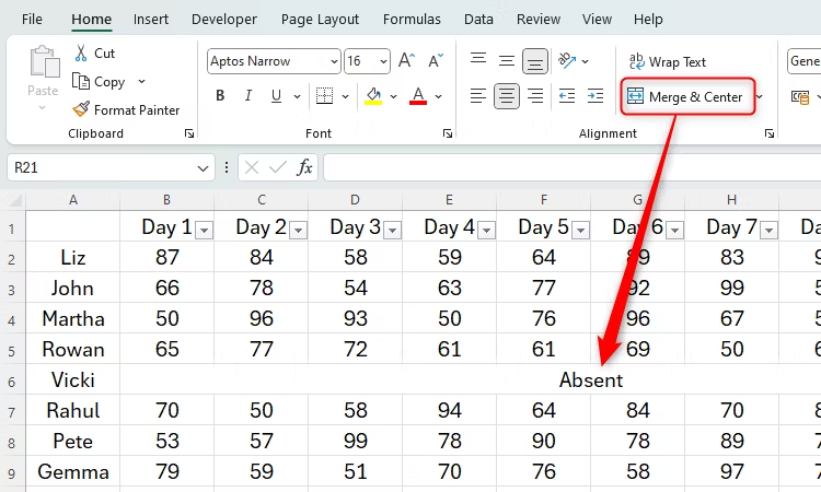
The Issue

However, merging cells causes issues when you try to perform actions with your data. This is mainly because many of Excel’s functions rely on you having a consistent setup of rows and columns, and merging cells causes your sheet to break this consistency.

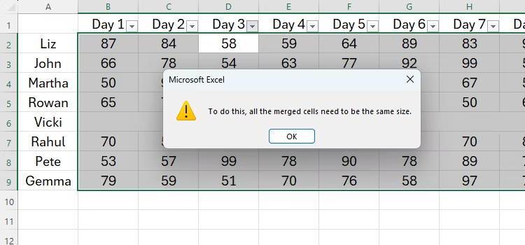
First, if you try to sort your data, you’ll receive an error message.

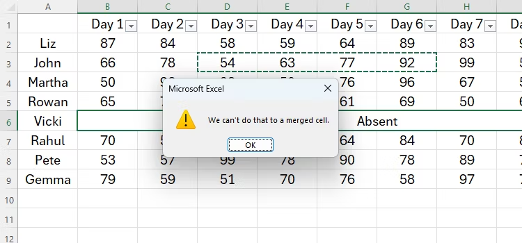
Likewise, you’ll encounter an issue if you try to paste data from an unmerged row to a merged row.

The Solution

First, click “Merge and Center” to unmerge the cells. Then, select the cells again, and click the icon in the bottom-right corner of the Alignment group in the Home tab.

Open the Horizontal drop-down menu in the Text Alignment section of the dialog box, click “Center Across Selection,” and click “OK.”

You will now see the text appear as it did when you used the Merge And Center option, but the cells’ structures and integrity have been retained.

“Center Across Selection” only works across rows, and not down columns.

Creating Tables Manually

Admittedly, before I became a power user of Excel, I didn’t realize the issues that creating and formatting tables manually would cause.

The Issue

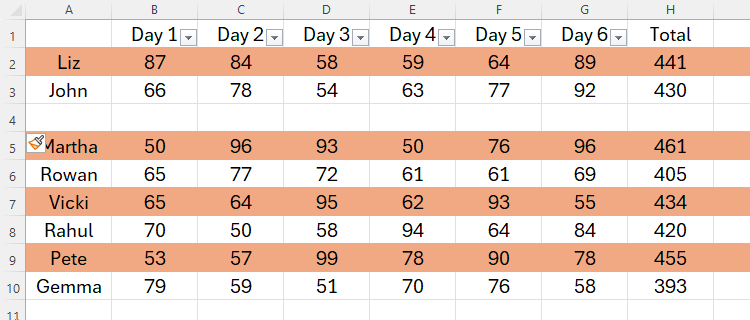
I used to format my data and copy formulas to new rows manually, but I always encountered issues if I wanted to add new rows or use my data to create a chart. For example, in the screenshot below, I have manually colored alternate rows—but when I add a new row, this affects my formatting, and I’d have to start all over again.

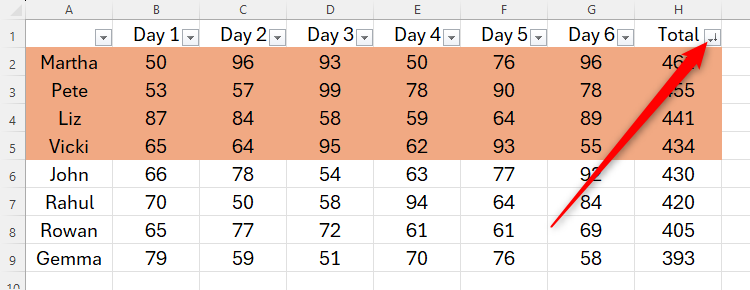
Similarly, if I add a filter to the columns, when I reorder the data, this will also mess up my formatting.

The Solution

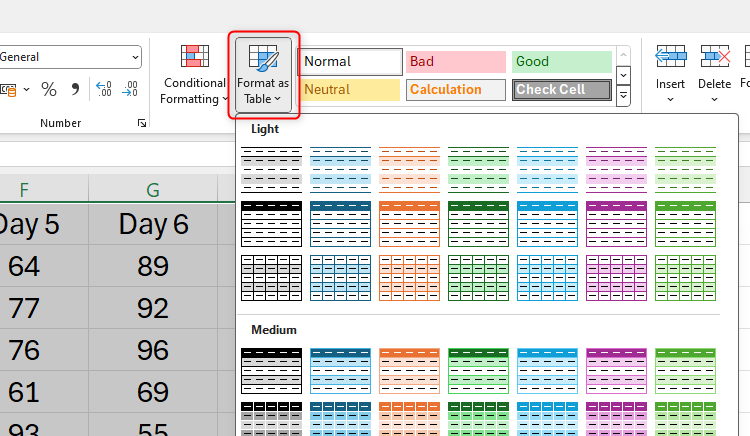
There’s a really easy way to deal with these issues. First, select all the data in your original, unformatted table, including your header columns and rows. Then, in the Home tab, click the Format As Table drop-down arrow, and choose a design that works for you.

To do the same in Excel for the web, select your data and click Insert > Table.

In the Create Table dialog box, check the “My Table Has Headers” checkbox if you have a header row at the top of your table, and click “OK.”

Give your table a name in the Table Design tab, so that you can refer to the table in formulas or jump to the table quickly using the name box.

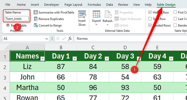
In the same tab, you can also change the Table Style and Table Style Options (such as including a filter button or banded rows), as well as a bunch of other actions to perfect your data presentation.

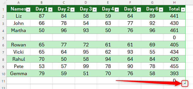
Now, if I were to add a row or column in the center of the table, the formatting would automatically update. I can also use the handle in the bottom-right corner of the table to add more rows to the bottom or columns to the right. Finally, Excel would automatically apply formulas to any new rows I add.

Overall, formatting your data as a table makes Excel aware that it’s not just a string of data, but instead should behave as a table, making everything a lot easier down the line.

Having Blank Rows and Columns

Many people (and, surprisingly, online Excel tutorials) leave row 1 and column A of their Excel sheets blank, probably because they think it makes their spreadsheets look better. This is probably due to the fact that in Microsoft Word, you can physically see the page borders, but you cannot in Excel until you preview your print layout.

The Issue

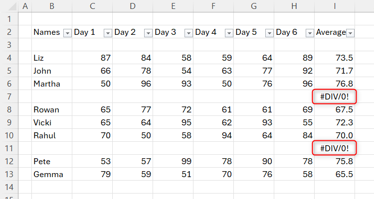
Aside from the fact that this is unnecessary, as Excel will automatically add page borders when you print your data, leaving rows and columns blank can cause other problems. For example, blank rows can disrupt your sorting and filtering, and they can also lead to formula issues and error messages when using AutoFill.

• ‘Baddest Lawyer’ Ifunanya clarifies controversy surrounding her professional status
• 10 notable Nigerians who recently joined the Guinness World Record book
• Adekunle Gold says he was ‘bullied’ for opening about sickle cell disease
• Bedtime stories: The saddest man in the room
• IPOB accuses military of secret abduction, torture of members

The Solution

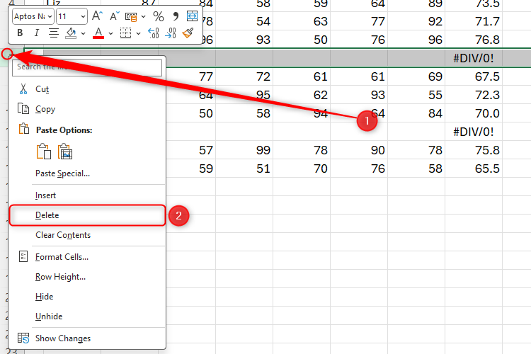
If you only have one or two blank rows or columns, you can right-click the row number or column letter and click “Delete.”

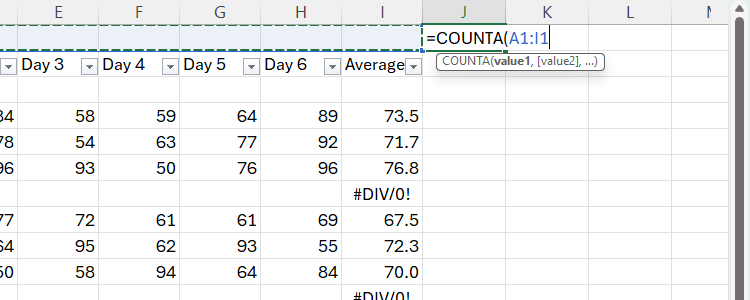
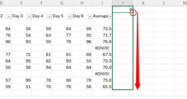
However, if you have lots of blank rows, you can use the COUNTA function to rectify this. Scroll across to the right until you reach the end of your data, and in cell 1, type

=COUNTA(

and select all the data to the left of that cell. Then, press Enter.

Next, drag the AutoFill handle to the bottom of your data.

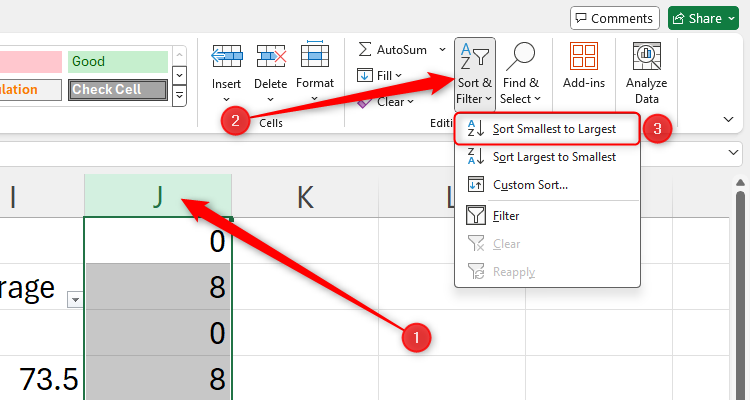
Now, select the whole column containing your COUNTA formulas, and in the Editing group on the Home tab, click the “Sort And Filter” drop-down arrow and click “Sort Smallest To Largest.”

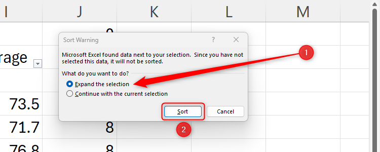
In the Sort Warning dialog box, choose “Expand The Selection” and click “Sort.”

You will then see all your blank rows move to the top, which you can select and delete.

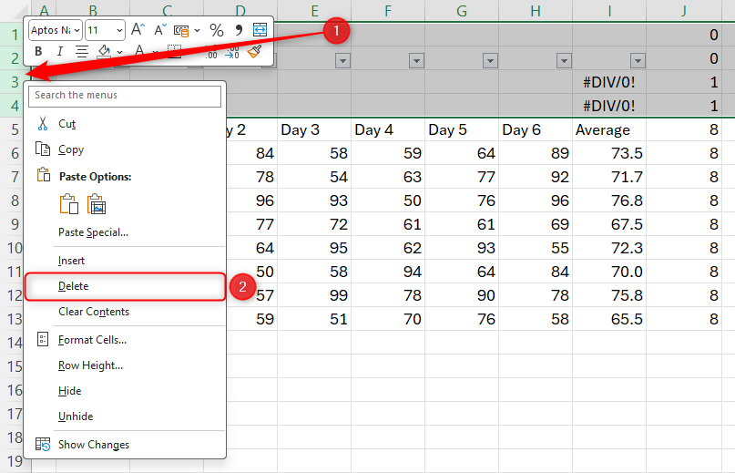
Finally, delete your COUNTA column.

Typing Sequences Manually

There are many circumstances in Excel that require you to present data sequentially, such as ascending numbers or date intervals.

The Issue

However, typing sequential data can be time-consuming and cause problems if you mistype a value or miss one out.

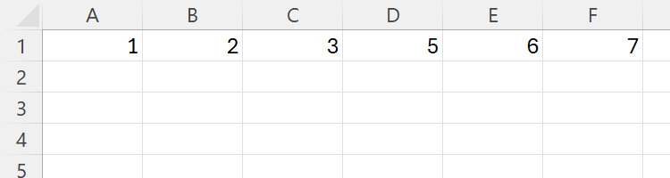
The Solution

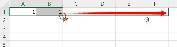
Excel’s AutoFill can recognize patterns in your data and fill in the rest for you. Start by typing the first two values in your data. Then, select these values and use the AutoFill handle to complete the data.

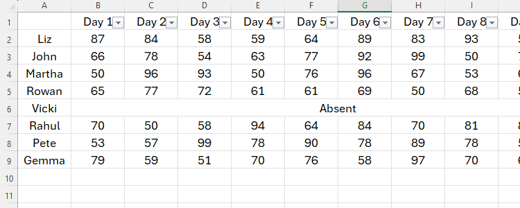
This will also work if your numbers are alongside other text in the cells (for example, Day 1, Day 2, and so on), and other sequential values such as dates.

Excel doesn’t recognize letters in the alphabet as a pattern, so use numbers if you want Excel to AutoFill the data for you.

Using the Wrong Reference Type

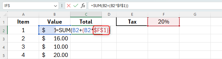
Referencing other cells in formulas is a great way to link your data together and update calculations automatically based on changing cell values. In this example, I have referenced cells B2 and F1 when calculating the total value in cell C2.

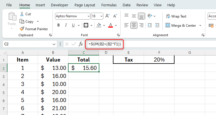
The Issue

However, many people encounter problems when using AutoFill, as they might not understand the different types of references in Excel.

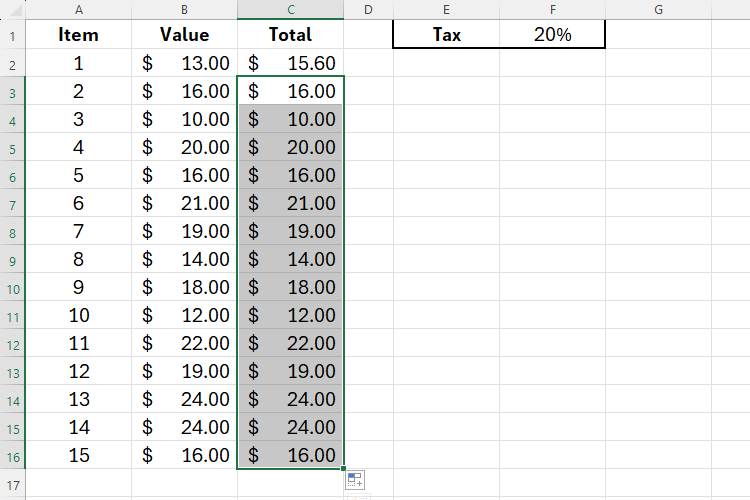
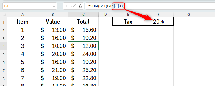
When I use AutoFill to calculate the totals for the remaining items, it doesn’t seem to have added the 20% tax to the values.

The Solution

There are three types of references in Excel, and it’s crucial you understand what they are and what they do if you want to copy calculations to other cells.

Relative references assess the relative positions between cells. In the example above, the initial calculation was made between cells C2 (where I typed my formula), B2 (one to the left of C2), and F1 (three to the right and one up from C2). When I copy this formula to cell C3, Excel will reference the cells in the same relative positions to where I am typing.

So, I would need to use an absolute reference to tell Excel to continually reference cell F1 when I AutoFill downwards. To do this, I would add dollar symbols before each part of the cell reference, or press F4 after typing or clicking the cell I want to reference.

Then, when I AutoFill the remaining totals, Excel will continue to reference F1 to make the calculation.

If I wanted to keep my row reference or column reference the same but let Excel adjust the other according to my formula’s location, I would use a mixed reference by typing the dollar symbol before the relevant part of my reference.

Not Locking Cells or Using Data Validation

Excel is great for creating a spreadsheet and then sharing it with others to add their data.

The Issue

However, if you share your sheet with someone who either isn’t very accustomed to Excel or has a habit of changing things you don’t want them to change, this could lead to your hard work being quickly undone.

The Solution

Excel lets you control what other people can enter into a spreadsheet through data validation and locked cells.

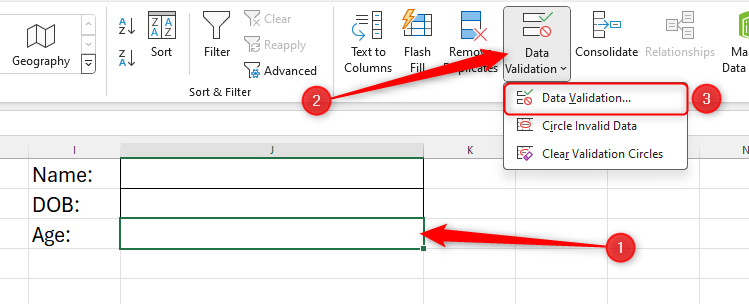
Data validation dictates what type of data can be input into a cell. Click the relevant cell or cells and, in the Data tab, go to the Data Tools group and click “Data Validation” in the Data Validation drop-down option.

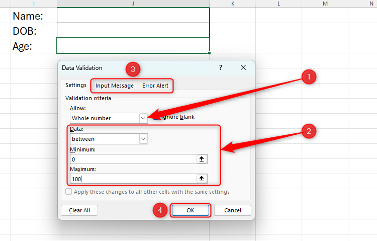
In the Validation Criteria section of the dialog box, click the “Allow” drop-down arrow and define the data type and range for the cell or cells. You can also have a message appear when someone clicks on those cells using the Input Message tab, and create a pop-up message if someone tries to input the wrong type of data using the Error Alert tab. When you’re done, click “OK.”

If you want to lock the cells you don’t want people to change at all, you can protect the worksheet. By default, when you protect the worksheet, all cells are locked, so you need to first choose which cells other people can click or edit.

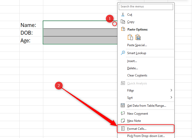
To do this, select and right-click those cells, and click “Format Cells.”

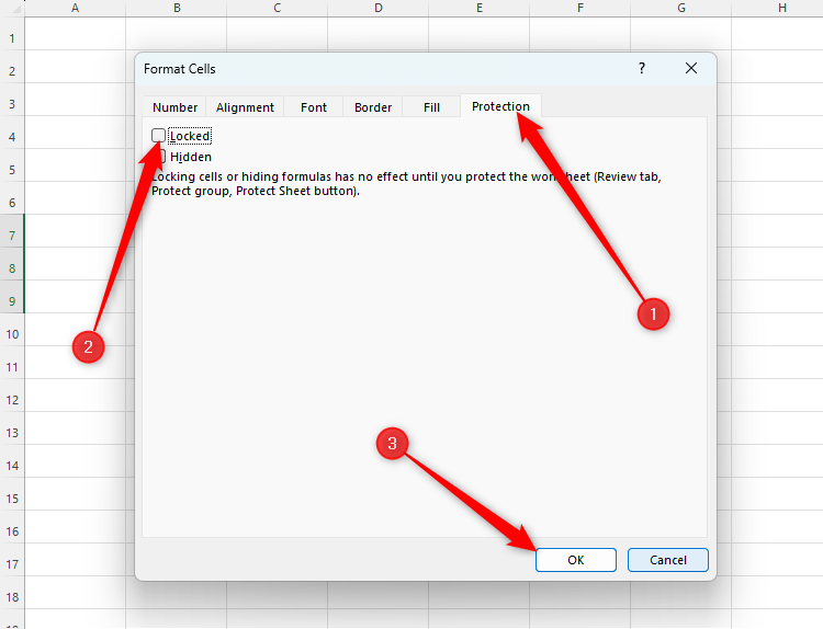
Then, in the Protection tab, uncheck “Locked,” and click “OK.”

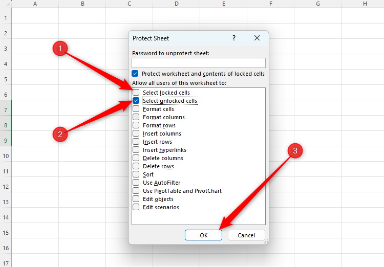
When you’re ready to send your sheet, click “Protect Sheet” in the Review tab, uncheck “Select Locked Cells”, and check “Select Unlocked Cells”. You can also enter a password if you wish. Then, click “OK.”

You will now see that only the cells you selected are clickable and editable.

To reverse this action, click “Unprotect Sheet.” If you password-protected your sheet earlier, you’ll need to type the password again to complete this action.

To do the same in Excel for the web, click “Protection” in the Review tab, and use the sidebar to choose which cells to unlock.